Introduction

The discrete logarithm problem is the basis for many public-key cryptographic algorithms. Suppose that we are given the numbers \(a\), \(b\), and a prime number \(p\), and have to find a number \(x\) such that \[b \equiv a^x \pmod p.\] Classically, this problem is considered difficult for suitable parameters. The method proposed by Shor for factorization can also be adapted to discrete logarithms (Shor 1994). The common part is the same: we have to construct a periodic object and extract its period by means of the quantum Fourier transform.

In this article we consider the ordinary discrete logarithm in the multiplicative group \((\mathbb{Z}/p\mathbb{Z})^\times\). This is the bridge between the factorization version of Shor’s algorithm and the elliptic-curve version, where the multiplicative group is replaced by a cyclic subgroup generated by a point on a curve.

The Function For The Discrete Logarithm

Let \[b \equiv a^x \pmod p,\] where \(p\) is prime and \(a\), \(b\), and \(p\) are known, while \(x\) is unknown. We work in the multiplicative group \[\mathbb{F}_p^\times=(\mathbb{Z}/p\mathbb{Z})^\times,\] and assume that \(a\) is a generator of this group. Its order is then \[q=p-1.\]

As in the factorization case, we have to construct a function whose period contains the unknown number. We choose the following function of two arguments: \[f(x_1,x_2) \equiv b^{x_1}a^{x_2} \equiv a^{x x_1+x_2} \pmod p. \label{eq:dlog-function}\]

Example.

Let us consider the problem \[\operatorname{ind}_3 14 \pmod {17},\] or, in other words, the equation \[3^x \equiv 14 \pmod {17}.\] Here \(p=17\), \(a=3\), and \(b=14\). The function [eq:dlog-function] has the form \[f(x_1,x_2)=14^{x_1}3^{x_2}\pmod {17}.\] It is shown in [fig:dlog-function].

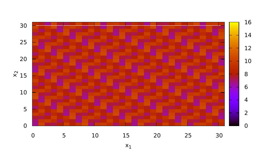
The number \(14\), just as \(3\), is a generator of \((\mathbb{Z}/17\mathbb{Z})^\times\). The answer to the discrete logarithm problem is \[14 \equiv 3^9 \pmod {17}.\] Thus the hidden value is \(x=9\). The function above is periodic in two directions, and these periods encode this number.

Measurement And Level Sets

As in Shor’s factorization algorithm, the function value is computed in a quantum register and then measured. Suppose that the measurement gives a value \(c\in(\mathbb{Z}/p\mathbb{Z})^\times\). Since \(a\) is a generator, there exists a number \(x_0\) such that \[c \equiv a^{x_0}\pmod p.\] Using Fermat’s little theorem, \[a^{p-1}\equiv 1 \pmod p,\] we can rewrite the condition \(f(x_1,x_2)=c\) as \[x x_1+x_2\equiv x_0 \pmod q,\] where \(q=p-1\).

Thus, after measuring the value register, only those pairs \((x_1,x_2)\) remain that lie on one of the level sets \[x_2\equiv x_0-x x_1\pmod q.\] If the function is shifted by a period vector, it remains on the same level set. Therefore the period relation contains the same number \(x\) that we are looking for.

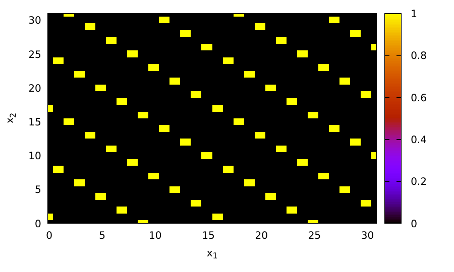
It is convenient to describe the post-measurement set by the indicator function \[f'(x_1,x_2)= \begin{cases} 1, & x x_1+x_2\equiv x_0 \pmod q,\\ 0, & x x_1+x_2\not\equiv x_0 \pmod q. \end{cases} \label{eq:level-indicator}\]

Example.

Continue the example with \(p=17\), \(a=3\), \(b=14\). Suppose that the measurement gives \[f(x_1,x_2)=3.\] Then \(3=3^{x_0}\), so \(x_0=1\). The remaining pairs satisfy \[9x_1+x_2\equiv 1 \pmod {16}.\] They are shown in [fig:dlog-level-set].

The Two-Dimensional Fourier Transform

Now we apply the Fourier transform to the function [eq:level-indicator]. For its Fourier image we have \[\tilde{f'}(j_1,j_2) =\frac{1}{M} \sum_{x_1=0}^{M-1}\sum_{x_2=0}^{M-1} f'(x_1,x_2) e^{-i\omega(x_1j_1+x_2j_2)}, \label{eq:two-dimensional-fourier}\] where \[\omega=\frac{2\pi}{M},\] and \(M\) is the number of samples in each coordinate.

First let us consider the case \[M=q.\] For every fixed \(x_1\), the value of \(x_2\) is determined modulo \(q\): \[x_2\equiv x_0-x x_1\pmod q.\] If the representative crosses zero, then we can write it as \[x_2=x_0+q-x x_1.\] However, for \(M=q\) this gives the same phase: \[\begin{aligned} e^{-i\omega x_2j_2} &=e^{-i\omega(x_0-x x_1+q)j_2} \nonumber \\ &=e^{-i\omega(x_0-x x_1)j_2-i\omega qj_2} \nonumber \\ &=e^{-i\omega(x_0-x x_1)j_2}. \label{eq:same-phase} \end{aligned}\] Thus both representatives can be reduced to the first one.

Continuing [eq:two-dimensional-fourier], we obtain \[\begin{aligned} \tilde{f'}(j_1,j_2) &=\frac{1}{M} \sum_{x_1=0}^{M-1} e^{-i\omega\left(x_1j_1+(x_0-x x_1)j_2\right)} \nonumber\\ &= \frac{1}{M}e^{-i\omega x_0j_2} \sum_{x_1=0}^{M-1} e^{-i\omega x_1(j_1-xj_2)}. \label{eq:fourier-level-set} \end{aligned}\]

The sum in [eq:fourier-level-set] is nonzero when \[j_1\equiv xj_2\pmod M. \label{eq:maximum-relation}\] Indeed, in that case every term in the sum is equal to \(1\). If \[j_1\not\equiv xj_2\pmod M,\] then the geometric progression gives \[\begin{aligned} \tilde{f'}(j_1,j_2) &= \frac{e^{-i\omega x_0j_2}}{M} \sum_{x_1=0}^{M-1} e^{-i\omega x_1(j_1-xj_2)} \nonumber\\ &= \frac{e^{-i\omega x_0j_2}}{M} \frac{ e^{-i\omega M(j_1-xj_2)}-1 }{ e^{-i\omega(j_1-xj_2)}-1 } \nonumber\\ &= \frac{e^{-i\omega x_0j_2}}{M} \frac{ e^{-i2\pi(j_1-xj_2)}-1 }{ e^{-i\omega(j_1-xj_2)}-1 } =0. \label{eq:fourier-zero} \end{aligned}\]

Therefore the maxima of the Fourier transform satisfy \[j_1\equiv xj_2\pmod M.\] If \(j_2\) is invertible modulo \(M\), then the unknown discrete logarithm can be recovered as \[x\equiv j_1j_2^{-1}\pmod M. \label{eq:dlog-recovery}\]

Remark.

If there exists a nonzero number \(y\) such that \[j_2y\equiv 0\pmod M,\] then \(j_2\) is a zero divisor in \(\mathbb{Z}/M\mathbb{Z}\). In this case \[\gcd(j_2,M)\ne 1,\] and \(j_2^{-1}\) does not exist. Then formula [eq:dlog-recovery] cannot be used with this particular Fourier maximum. We have to use another maximum.

The Exact Example

Let us return to \[3^x\equiv 14\pmod {17}.\] Here \(M=q=16\). The Fourier image of the function from [fig:dlog-level-set] is shown in [fig:dlog-fourier-exact].

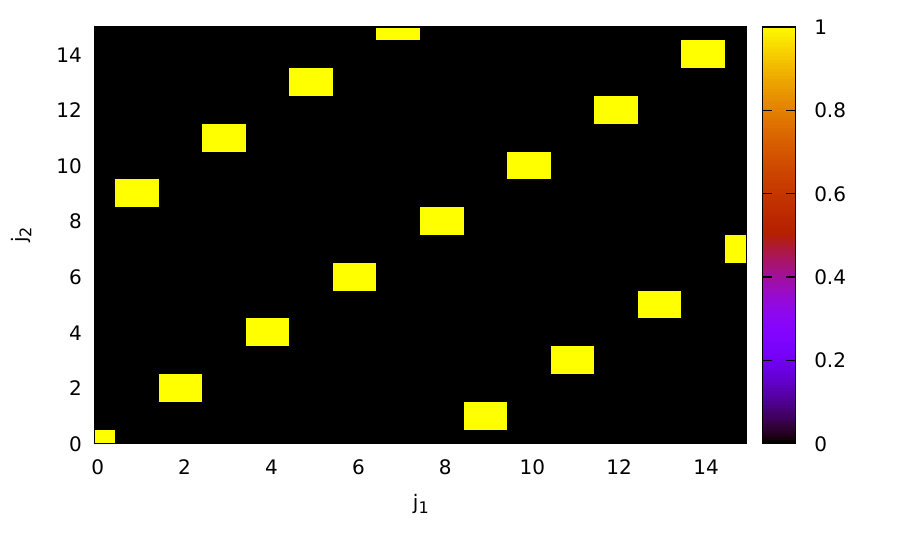
The lower maxima follow with interval \(T_{j_1}=9\) in the \(j_1\) coordinate and \(T_{j_2}=1\) in the \(j_2\) coordinate. Therefore we can take \[j_1=9,\qquad j_2=1.\] By [eq:dlog-recovery], \[x\equiv 9\cdot 1^{-1}\equiv 9\pmod {16}.\] This is the expected solution of the equation \[3^x\equiv 14\pmod {17}.\]

The same result can be obtained from another maximum. For example, take \[j_1=11,\qquad j_2=3.\] Since \[3\cdot 11=33\equiv 1\pmod {16},\] we have \[j_2^{-1}\equiv 11\pmod {16}.\] Thus \[x\equiv 11\cdot 11\equiv 121\equiv 9\pmod {16}.\]

It is worth noting that points on the diagonal do not necessarily give a valid answer. For example, for \[j_1=6,\qquad j_2=6,\] we have \[\gcd(6,16)=2\ne 1.\] Therefore \(6^{-1}\) does not exist modulo \(16\), and this maximum cannot be used in [eq:dlog-recovery].

Approximate Examples

The previous example was especially convenient because the number of samples was exactly equal to the group order: \[M=q.\] In the quantum algorithm \(M\) is usually a power of two. If \(M\ne q\), but \(M\) is close to \(q\), then the coordinates of the Fourier maxima give approximations to the same relation. This is the cyclic-group situation used in Shor’s discrete logarithm algorithm (Shor 1994); the elliptic-curve version uses the same idea with the group of curve points and is analyzed in (Proos and Zalka 2003).

Example.

Consider the equation \[2^x\equiv 14\pmod {59}.\] The number \(2\) is a generator of \(\mathbb{F}_{59}^{\times}\), and the solution is \[x=19.\] We take \[M=64\approx q=p-1=58.\] The function under investigation is \[f(x_1,x_2)=14^{x_1}2^{x_2}\pmod {59}.\] Suppose that the measured value is \[f(x_1,x_2)=2^{50}\equiv 3\pmod {59},\] so \(x_0=50\). The Fourier image of the corresponding indicator function is shown in [fig:dlog-fourier-mod59].

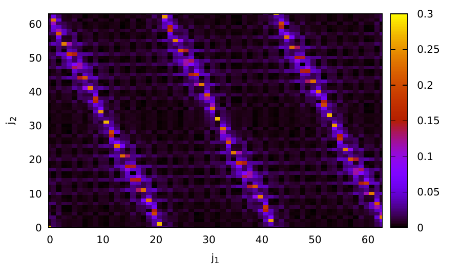
The three lower maxima have approximate coordinates \[(j_1,j_2)\approx (20,1),\quad (41,2.2),\quad (62,3).\] Therefore \[\frac{j_1}{j_2}\approx 20,\quad 18.6,\quad 20.6.\] These values are close to the exact answer \(x=19\).

Example.

Now consider \[3^x\equiv 14\pmod {19}.\] The function is \[f(x_1,x_2)=14^{x_1}3^{x_2}\pmod {19}.\] Suppose that the measurement gives \[f(x_1,x_2)=3,\] so \(x_0=1\). Again we take \(M=64\). Since \[q=p-1=18\] does not divide \(64\), the Fourier image gives an approximation. It is shown in [fig:dlog-fourier-mod19].

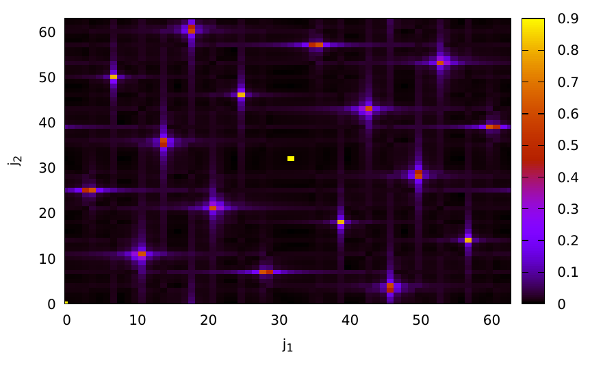
The lowest maximum has approximate coordinates \[j_1=46,\qquad j_2=3.5.\] Thus \[x\approx \frac{46}{3.5}\approx 13.14.\] The exact solution is \(x=13\), so the approximation points to the correct discrete logarithm.

Two-Dimensional Quantum Fourier Transform

To determine periods of functions of two arguments, we can use a two-dimensional quantum Fourier transform. It can be built from two ordinary one-dimensional Fourier transforms, as shown in [fig:qft-2d-circuit].

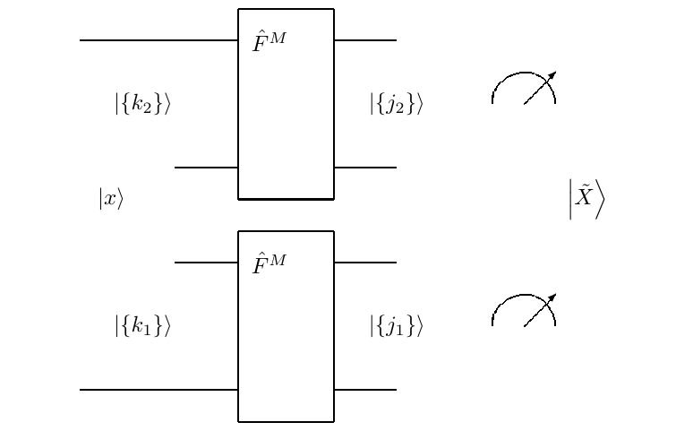
Let us first consider the simple tensor-product case \[\ket{x}=\ket{x}_1\otimes\ket{x}_2,\] where \[\ket{x}_{1,2} =\sum_{k_{1,2}=0}^{M-1} x^{(1,2)}_{k_{1,2}}\ket{k_{1,2}}.\] After applying the Fourier transform to both registers, we get \[\ket{\tilde{X}} =\ket{\tilde{X}_1}\otimes\ket{\tilde{X}_2},\] where \[\ket{\tilde{X}_{1,2}} =\sum_{j_{1,2}=0}^{M-1} \tilde{X}^{(1,2)}_{j_{1,2}}\ket{j_{1,2}}.\] For each coordinate, \[\tilde{X}^{(1,2)}_{j_{1,2}} =\frac{1}{\sqrt M} \sum_{k_{1,2}=0}^{M-1} e^{-i\omega k_{1,2}j_{1,2}} x^{(1,2)}_{k_{1,2}}.\] Therefore \[\begin{aligned} \ket{\tilde{X}} &= \sum_{j_1=0}^{M-1}\sum_{j_2=0}^{M-1} \tilde{X}^{(1)}_{j_1} \tilde{X}^{(2)}_{j_2} \ket{j_1}\otimes\ket{j_2} \nonumber\\ &= \sum_{j_1=0}^{M-1}\sum_{j_2=0}^{M-1} \tilde{X}_{j_1,j_2} \ket{j_1}\otimes\ket{j_2}, \label{eq:qft-2d-state} \end{aligned}\] where \[\begin{aligned} \tilde{X}_{j_1,j_2} &= \frac{1}{(\sqrt M)^2} \sum_{k_1=0}^{M-1}\sum_{k_2=0}^{M-1} e^{-i\omega(k_1j_1+k_2j_2)} x^{(1)}_{k_1}x^{(2)}_{k_2} \nonumber\\ &= \frac{1}{M} \sum_{k_1=0}^{M-1}\sum_{k_2=0}^{M-1} e^{-i\omega(k_1j_1+k_2j_2)} x_{k_1,k_2}. \label{eq:qft-2d-amplitudes} \end{aligned}\]

Thus two one-dimensional quantum Fourier transforms give the two-dimensional Fourier transform of the amplitudes. By linearity, the same formula is used for a general two-register state \[\ket{x} = \sum_{k_1=0}^{M-1}\sum_{k_2=0}^{M-1} x_{k_1,k_2}\ket{k_1}\otimes\ket{k_2}.\]

Period Finding For Two Arguments

The period-finding circuit for a function of two arguments is shown in [fig:period-finding-2d-circuit]. The first two registers are put into uniform superposition, the function is computed, and the function register is measured. This measurement leaves a set of pairs \((x_1,x_2)\) satisfying one level-set relation. Then the two-dimensional quantum Fourier transform is applied to the two argument registers.

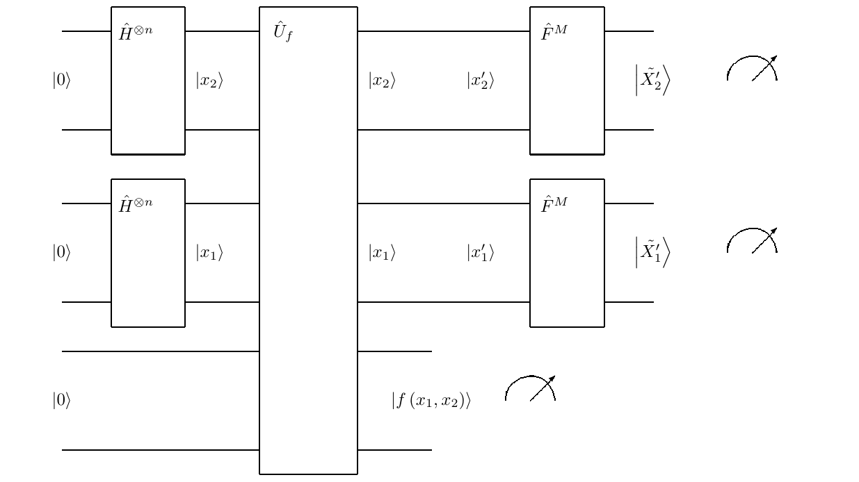
The measured Fourier coordinates \((j_1,j_2)\) identify maxima of the two-dimensional Fourier image. In the exact case these maxima satisfy \[j_1\equiv xj_2\pmod M.\] Therefore, when \(j_2\) is invertible modulo \(M\), the hidden number is recovered from \[x\equiv j_1j_2^{-1}\pmod M.\] When \(M\) is only close to the group order, the same coordinates give an approximation, and the classical post-processing step recovers the discrete logarithm with high probability (Nielsen and Chuang 2000).

Conclusion

The ordinary discrete logarithm problem can be reduced to the extraction of a linear period relation. We begin with \[b\equiv a^x\pmod p\] and construct \[f(x_1,x_2)=b^{x_1}a^{x_2}.\] After measuring the function value, the remaining pairs satisfy \[x x_1+x_2\equiv x_0\pmod q.\] The two-dimensional Fourier transform turns this level-set structure into maxima satisfying \[j_1\equiv xj_2\pmod M.\] This gives the discrete logarithm by the formula \[x\equiv j_1j_2^{-1}\pmod M\] in the exact case, and by approximation when the sampling size is close to the group order. The elliptic-curve case uses the same mechanism, but the multiplicative group is replaced by a cyclic subgroup of an elliptic curve.